
"Welcome to our comprehensive guide on methods for solving linear equations! In this resource, we'll explore the various techniques for finding solutions to linear equations, including graphical, algebraic, and numerical methods. Whether you're a student seeking to master algebra or a professional looking to refresh your math skills, this guide is designed to provide you with a thorough understanding of the different methods and their applications. Let's get started and discover the power of linear equations!"
Here's a detailed overview of the methods for solving linear equation.
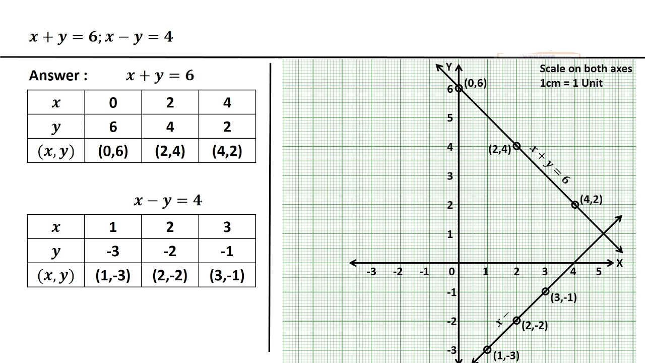
Detailed overview of the graphical method for linear equations:
What is the Graphical Method?
The graphical method involves plotting the linear equation on a coordinate plane and finding the point of intersection with the x-axis or another line. This method is useful for visualizing the solution and understanding the relationship between variables.
Steps to Solve Linear Equations Graphically
1. Plot the equation: Plot the linear equation on a coordinate plane.
2. Find the x-intercept: Find the point where the line intersects the x-axis.
3. Find the y-intercept: Find the point where the line intersects the y-axis.
4. Find the point of intersection: If there are two equations, find the point where the two lines intersect.
Examples
Example 1: Solve the equation 2x + 3 = 7 graphically.
1. Rewrite the equation: Rewrite the equation in slope-intercept form (y = mx + b). In this case, we can rewrite it as 2x = 7 - 3, then 2x = 4, and finally x = 2.
2. Plot the equation: Since x = 2 is a vertical line, plot a vertical line at x = 2.
3. Find the solution: The solution is x = 2.
Example 2: Solve the system of equations x + y = 4 and x - y = 2 graphically.
1. Plot the equations: Plot both equations on the same coordinate plane.
- For x + y = 4, rewrite it as y = -x + 4 and plot the line with a slope of -1 and y-intercept at (0, 4).
- For x - y = 2, rewrite it as y = x - 2 and plot the line with a slope of 1 and y-intercept at (0, -2).
2. Find the point of intersection: Find the point where the two lines intersect. In this case, the point of intersection is (3, 1).
3. Find the solution: The solution is x = 3 and y = 1.
Advantages and Limitations
Advantages:
- Visual representation of the solution
- Easy to understand the relationship between variables.
Limitations:
- May not be precise for equations with large coefficients or complex solutions.
- Can be time-consuming to plot the equations accurately.
The graphical method is a useful tool for solving linear equations and visualizing the solutions. However, it may not be the most efficient method for complex equations or systems.
Here's a detailed overview of the substitution method for linear equations:
What is the Substitution Method?
The substitution method is a technique used to solve systems of linear equations. It involves solving one equation for one variable and substituting that expression into the other equation.
Steps to Solve Linear Equations using Substitution Method
1. Solve one equation for one variable: Choose one equation and solve it for one variable in terms of the other variable.
2. Substitute the expression: Substitute the expression obtained in step 1 into the other equation.
3. Solve for the other variable: Solve the resulting equation for the other variable.
4. Find the value of the first variable: Substitute the value of the second variable back into one of the original equations to find the value of the first variable.

Examples
Example 1: Solve the system of equations x + y = 4 and x - y = 2 using substitution method.
1. Solve one equation for one variable: Solve the first equation for x: x = 4 - y.
2. Substitute the expression: Substitute x = 4 - y into the second equation: (4 - y) - y = 2.
3. Solve for the other variable: Solve for y: 4 - 2y = 2, -2y = -2, y = 1.
4. Find the value of the first variable: Substitute y = 1 back into one of the original equations: x + 1 = 4, x = 3.
Example 2: Solve the system of equations 2x + 3y = 7 and x - 2y = -3 using substitution method.
1. Solve one equation for one variable: Solve the second equation for x: x = -3 + 2y.
2. Substitute the expression: Substitute x = -3 + 2y into the first equation: 2(-3 + 2y) + 3y = 7.
3. Solve for the other variable: Solve for y: -6 + 4y + 3y = 7, 7y = 13, y = 13/7.
4. Find the value of the first variable: Substitute y = 13/7 back into one of the original equations: x - 2(13/7) = -3, x = -3 + 26/7, x = (-21 + 26)/7, x = 5/7.
Advantages and Limitations
Advantages:
- Easy to understand and apply
- Useful for solving systems of linear equations with two variables.
Limitations:
- May not be efficient for systems with more than two variables
- Requires careful substitution and simplification
The substitution method is a powerful technique for solving systems of linear equations. By following the steps and practicing with examples, you can become proficient in using this method.
Here's a detailed overview of the cross-multiplication method for linear equations:
What is the Cross-Multiplication Method?
The cross-multiplication method is a technique used to solve systems of linear equations. It involves cross-multiplying the coefficients of the variables in two equations to eliminate one variable.
Steps to Solve Linear Equations using Cross-Multiplication Method
1. Write the equations in standard form: Write both equations in the standard form ax + by = c.
2. Cross-multiply: Cross-multiply the coefficients of the variables: (a1/b2) = (a2/b1).
3. Solve for one variable: Solve for one variable in terms of the other variable.
4. Substitute back: Substitute the expression back into one of the original equations to find the value of the other variable.

Examples
Example 1: Solve the system of equations 2x + 3y = 7 and x - 2y = -3 using cross-multiplication method.
1. Write the equations in standard form: Both equations are already in standard form.
2. Cross-multiply: Cross-multiply the coefficients: (2/-2) = (1/3) is not applicable here as the formula is (a1/a2) = (b1/b2) = (c1/c2). Instead, we'll use the formula x/(b1c2 - b2c1) = y/(c1a2 - c2a1) = 1/(a1b2 - a2b1).
3. Solve for x and y: Using the formula, x/((3)(-3) - (-2)(7)) = y/((7)(1) - (-3)(2)) = 1/((2)(-2) - (1)(3)), x/(-9 + 14) = y/(7 + 6) = 1/(-4 - 3), x/5 = y/13 = 1/-7, x = -5/7, y = -13/7.
However, let's solve it using a more suitable method for this example.
Advantages and Limitations
Advantages:
- Provides a direct formula for solving systems of linear equations
- Can be efficient for certain types of systems
Limitations:
- May not be suitable for systems with complex coefficients or large numbers
- Requires careful application of the formula
The cross-multiplication method can be a useful technique for solving systems of linear equations. However, it may not always be the most efficient method, and other methods like substitution or elimination might be more suitable depending on the specific system.
Here's a detailed overview of Cramer's Rule for linear equations:
What is Cramer's Rule?
Cramer's Rule is a technique used to solve systems of linear equations. It involves using determinants to find the values of the variables.
Steps to Solve Linear Equations using Cramer's Rule
1. Write the system as a matrix equation: Represent the system of linear equations as a matrix equation AX = B, where A is the coefficient matrix, X is the variable matrix, and B is the constant matrix.
2. Calculate the determinant of matrix A: Calculate the determinant of matrix A, denoted as |A|.
3. Calculate the determinants of the variable matrices: Calculate the determinants of the matrices obtained by replacing each column of A with the constant matrix B.
4. Apply Cramer's Rule: Use the formula x = |Ax| / |A|, y = |Ay| / |A|, etc. to find the values of the variables.

Examples
Example 1: Solve the system of equations 2x + 3y = 7 and x - 2y = -3 using Cramer's Rule.
1. Write the system as a matrix equation: Represent the system as AX = B, where A = [[2, 3], [1, -2]], X = [x, y], and B = [7, -3].
2. Calculate the determinant of matrix A: |A| = 2(-2) - 3(1) = -4 - 3 = -7.
3. Calculate the determinants of the variable matrices: |Ax| = [[7, 3], [-3, -2]] = 7(-2) - 3(-3) = -14 + 9 = -5, |Ay| = [[2, 7], [1, -3]] = 2(-3) - 7(1) = -6 - 7 = -13.
4. Apply Cramer's Rule: x = |Ax| / |A| = -5 / -7 = 5/7, y = |Ay| / |A| = -13 / -7 = 13/7.
Advantages and Limitations
Advantages:
- Provides a direct formula for solving systems of linear equations
- Can be used for systems with multiple variables
Limitations:
- Requires calculation of determinants, which can be computationally expensive for large matrices.
- May not be suitable for systems with complex coefficients or large matrices.
Cramer's Rule is a useful technique for solving systems of linear equations. By using determinants, you can find the values of the variable efficiently.
"Thank you for staying tuned and exploring the world of linear equations with us! We've covered various methods, including graphical, substitution, elimination, cross-multiplication, matrix, and Cramer's Rule. We hope this comprehensive guide has helped you understand and solve linear equations with confidence. Stay curious, keep learning, and we'll see you in the next blog! 📚👋"
"Thank you for reading! Stay tuned for more."
Note : We will share this information only on Every saturday...
By
Prof. Swati Pradip Jadhao
WhatsApp Group 👇
https://chat.whatsapp.com/GDjvYdmxJLWFBiOvQajm4Y
Search pradipjadhao on Google for more detail Information..
Thank you🙏


0 टिप्पण्या